10 min to read
Databricks Step by Step: Build a Data Pipeline
Raw JSON files land in a folder every hour. By lunch, someone wants a dashboard. Here's the pipeline in between.
Every data team gets the same request eventually.
Order files are landing in cloud storage. Nobody cleans them. Somebody in sales wants revenue by product, every morning, without asking an engineer. And whatever you build has to keep working when tomorrow’s files show up with a missing date field.
This is the first post in Databricks Step by Step, a series where each post builds one common thing on Databricks from start to finish. If you’re new to the platform, start with Databricks in One Post for the background. This post builds the foundation everything else stands on: a pipeline that turns raw files into clean, trustworthy tables.
What We’re Building
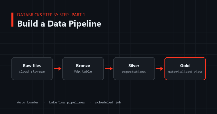
The pattern is called the medallion architecture. It sounds fancier than it is. It’s three layers of tables, each one cleaner than the last:
 Raw JSON files ──► BRONZE ──────► SILVER ──────────► GOLD
 (cloud storage)    exactly as     cleaned, typed,    business-ready
                    it arrived     bad rows dropped   aggregates
- Bronze keeps the raw data exactly as it arrived. If something goes wrong downstream, you can always rebuild from here.
- Silver is cleaned: proper types, one row per thing, bad records filtered out.
- Gold answers a business question. Revenue by product by day.
We’ll use a dataset that ships with every Databricks workspace, /databricks-datasets/retail-org/sales_orders, so you can follow along without bringing your own data.
The tools:
- Auto Loader reads new files from storage incrementally. It remembers what it has already processed, so each run only picks up what’s new.
- Lakeflow pipelines (the product formerly called Delta Live Tables) let you declare tables as Python functions. Databricks works out the order, the retries, and the infrastructure.
- Expectations are data quality rules attached to a table.
- Jobs run the whole thing on a schedule.
Step 1: Set Up a Home for the Tables
Everything in Databricks lives in Unity Catalog under a three-part name: catalog.schema.table. Create a schema for this project. Open a SQL editor or notebook and run:
CREATE SCHEMA IF NOT EXISTS main.retail;
If your workspace uses a different catalog than main, swap in its name here and everywhere below.
Step 2: Create the Pipeline
In the Databricks sidebar, go to Jobs & Pipelines → Create → ETL pipeline. Give it a name like retail-orders, and set the default catalog to main and the schema to retail. Databricks creates a pipeline with a code file for you to edit.
Pipeline code is different from a normal notebook. You don’t run it top to bottom. You declare tables, and the pipeline figures out the dependencies and runs them in the right order. Every pipeline file starts with the same import:
from pyspark import pipelines as dp
from pyspark.sql import functions as F
Step 3: Bronze, Ingesting Raw Files with Auto Loader
@dp.table(
    name="orders_bronze",
    comment="Raw sales orders, exactly as they arrived.",
)
def orders_bronze():
    return (
        spark.readStream
        .format("cloudFiles")                     # this is Auto Loader
        .option("cloudFiles.format", "json")
        .load("/databricks-datasets/retail-org/sales_orders")
        .withColumn("_ingested_at", F.current_timestamp())
        .withColumn("_source_file", F.col("_metadata.file_path"))
    )
The decorator turns this function into a streaming table. Because it reads with spark.readStream and cloudFiles, it’s incremental: the first run reads every file in the folder, and each run after that reads only the files that are new since the last run.
The two extra columns are a habit worth keeping. When someone asks “where did this weird row come from?” six months from now, _source_file and _ingested_at answer it in one query.
Step 4: Silver, Cleaning with Data Quality Rules
The raw orders have a few problems. The order time is a Unix timestamp stored as a string, and each order holds its products in a nested list. Silver fixes both and enforces some rules:
@dp.table(
    name="orders_silver",
    comment="One row per product per order, typed and validated.",
)
@dp.expect_or_drop("valid_order_number", "order_number IS NOT NULL")
@dp.expect_or_drop("valid_order_time", "order_ts IS NOT NULL")
@dp.expect("positive_quantity", "quantity > 0")
def orders_silver():
    return (
        spark.readStream.table("orders_bronze")
        .withColumn("order_ts", F.from_unixtime(F.col("order_datetime").cast("long")).cast("timestamp"))
        .withColumn("product", F.explode("ordered_products"))
        .select(
            "order_number",
            "customer_id",
            "order_ts",
            F.col("product.id").alias("product_id"),
            F.col("product.name").alias("product_name"),
            F.col("product.price").cast("double").alias("unit_price"),
            F.col("product.qty").cast("int").alias("quantity"),
        )
        .withColumn("line_total", F.col("unit_price") * F.col("quantity"))
    )
Those decorators are the expectations, and they’re the part that makes a pipeline trustworthy:
| Decorator | What happens when a row breaks the rule |
|---|---|
@dp.expect |
Row is kept; the violation is counted in the pipeline’s metrics |
@dp.expect_or_drop |
Row is dropped and counted |
@dp.expect_or_fail |
The whole update stops |
Pick based on the cost of being wrong. A missing order number makes a row useless, so drop it. A zero quantity is suspicious but might be legitimate (a free promo item, say), so keep it and watch the count. Use expect_or_fail for things that mean the source is badly broken, like a file with no columns you recognize.
Notice that silver reads orders_bronze by name. That reference is how the pipeline knows bronze must run first. You never write the run order yourself.
Step 5: Gold, Answering the Business Question
@dp.materialized_view(
    name="daily_product_revenue",
    comment="Revenue and units by product by day.",
)
def daily_product_revenue():
    return (
        spark.read.table("orders_silver")
        .groupBy(F.to_date("order_ts").alias("order_date"), "product_name")
        .agg(
            F.sum("line_total").alias("revenue"),
            F.sum("quantity").alias("units_sold"),
            F.countDistinct("order_number").alias("orders"),
        )
    )
This one is a materialized view, not a streaming table. The difference matters:
- A streaming table processes each new row once. That’s right for bronze and silver, where data only gets appended.
- A materialized view always reflects the current state of its inputs. That’s right for aggregates. If a late order arrives for last Tuesday, last Tuesday’s revenue needs to change, and a materialized view handles that for you.
A simple rule of thumb: streaming tables for ingesting and cleaning, materialized views for summarizing.
Step 6: Run It
Click Run pipeline. Databricks draws the dependency graph as it runs:
orders_bronze ──► orders_silver ──► daily_product_revenue
When it finishes, click each table to see row counts and, for silver, how many rows each expectation dropped or flagged. That data quality panel is worth checking after every change you make.
Then query the result like any other table:
SELECT order_date, product_name, revenue, units_sold
FROM main.retail.daily_product_revenue
ORDER BY order_date DESC, revenue DESC
LIMIT 20;
Run the pipeline a second time and watch the bronze row count. It doesn’t double, because Auto Loader already knows those files were processed. That’s incremental processing doing its job.
Step 7: Put It on a Schedule
A pipeline you have to remember to click isn’t a pipeline. From the pipeline page, click Schedule, choose a time (say, 6:00 AM daily), and save. Databricks creates a job that runs the pipeline for you.
If you’d rather keep the schedule in code, where it can be reviewed and versioned, the Databricks SDK can create the same job:
from databricks.sdk import WorkspaceClient
from databricks.sdk.service import jobs

w = WorkspaceClient()

w.jobs.create(
    name="retail-orders-daily",
    tasks=[
        jobs.Task(
            task_key="refresh_pipeline",
            pipeline_task=jobs.PipelineTask(pipeline_id="<your-pipeline-id>"),
        )
    ],
    schedule=jobs.CronSchedule(
        quartz_cron_expression="0 0 6 * * ?",   # 6:00 AM every day
        timezone_id="America/New_York",
    ),
    email_notifications=jobs.JobEmailNotifications(on_failure=["you@example.com"]),
)
The pipeline ID is on the pipeline’s settings page. Turn on failure emails either way. You want to hear about a failed run before the sales team does.
What Can Go Wrong
The pipeline can’t find a table. Inside a pipeline, refer to other pipeline tables by their short name (orders_silver). For tables outside the pipeline, use the full three-part name.
Expectations drop far more rows than you expected. Look at the dropped-row counts before you loosen a rule. A sudden spike usually means the source changed its format, which is exactly what the rule is there to catch.
A column changes type upstream. Auto Loader tracks the schema it has seen and handles new columns for you. A column that changes type is where a silver-layer cast earns its keep, because it keeps the mess out of everything downstream.
You need to reprocess everything. Run a full refresh from the pipeline page. It clears the tables and rebuilds them from the source files, which is why keeping raw data in bronze matters.
Where This Goes Next
You now have clean, scheduled, quality-checked tables, which is the starting point for nearly everything else on Databricks. Dashboards read from gold. Machine learning trains on silver. AI apps search over documents stored the same way.
Next in the series: training a machine learning model and registering it in Unity Catalog, so it’s tracked, versioned, and ready to deploy.